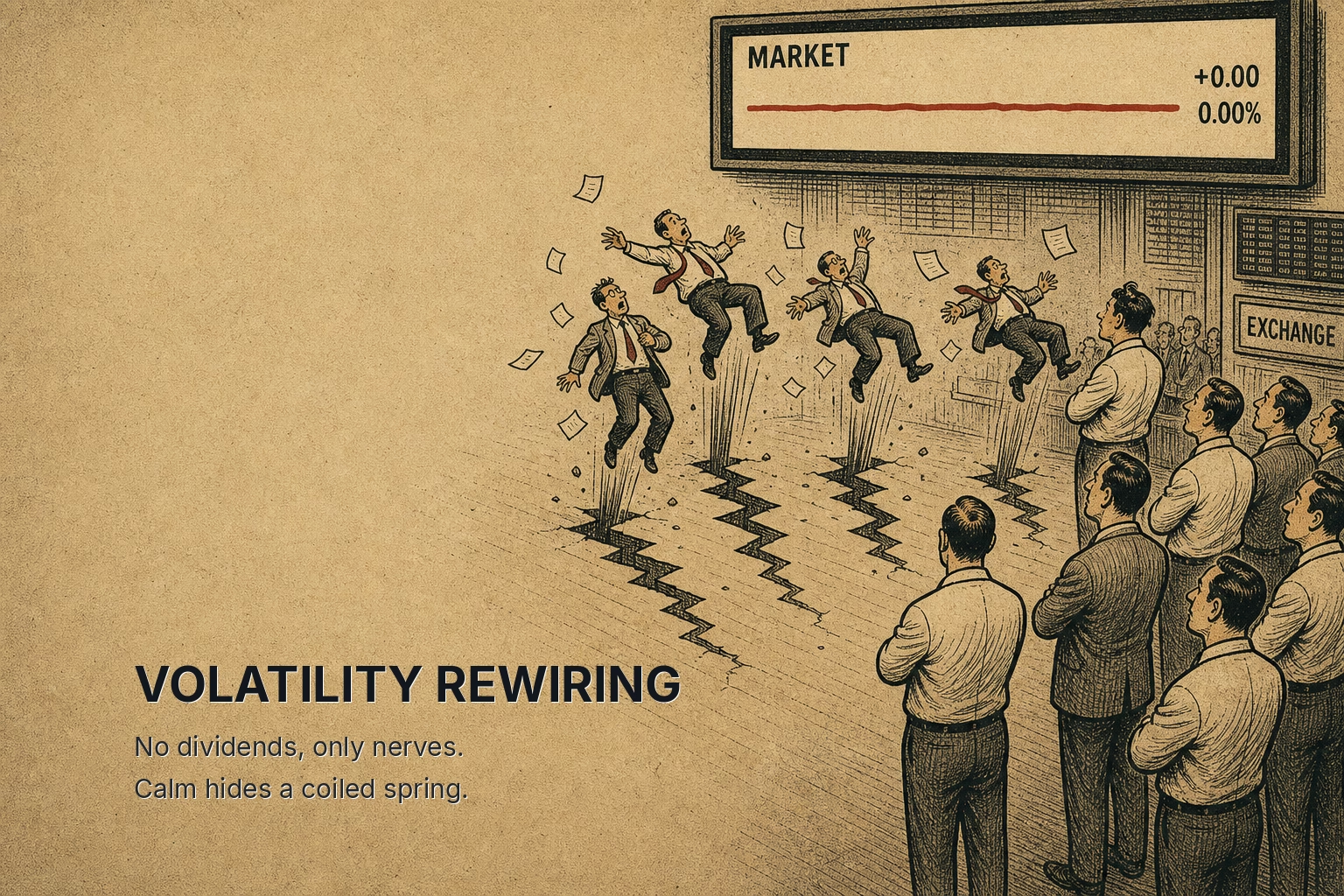
The most predictable seller in the equity market is not a panicked human. It is a fund that sells because it is disciplined, on a timetable that anyone with a calculator and a price history can reconstruct before the orders hit the tape.
The afternoon the calm broke, February 2018
On February 5, 2018, the Dow Jones Industrial Average fell 1,175 points, then its largest point decline on record. The VIX, the market's gauge of expected S&P 500 volatility over the next 30 days, closed at 37.32 after closing at 17.31 the session before. That 116% jump was the largest one-day percentage rise in the index's history. That evening, an exchange-traded note built to profit from low volatility lost roughly 96% of its value and was later shut down.
The short-volatility products drew the headlines. The more instructive part of the episode came afterward. The S&P 500 did not bottom on February 5. It kept falling through the following days and set its low on February 8, even though no new macro shock arrived in between. Prices were being pushed by mechanical selling from funds whose rules had just been triggered.
The fund family that explains that drift is the volatility-targeting fund, a portfolio that sizes its equity exposure to keep its own expected volatility near a fixed number. Before February 2018, markets had spent most of 2017 in historically quiet conditions. Quiet conditions told these funds to hold more equity. One violent day told them to hold far less. The practical lesson from the episode is that the first day of a volatility shock is the news, and the next several days are often the arithmetic.
The rule that turns calm into leverage
A volatility-targeting fund runs one core equation:
Equity exposure = Target volatility / Realized volatility
Realized volatility is the annualized standard deviation of recent daily returns, measured over a fixed lookback window. A common choice is 20 trading days, roughly one month. The target is the risk level the fund promises its holders, often 10% a year.
Take a fund targeting 10% volatility. If the market has been moving with 8% annualized realized volatility, the rule says to hold 10/8, or 125% of capital in equities. The fund borrows or uses futures to get there. Most products cap leverage, frequently at 150%, so a very quiet market pins them at the ceiling.
Now let realized volatility rise to 16%. The rule gives 10/16, or 62.5%. On a $100 billion book, exposure falls from $125 billion to $62.5 billion. The fund has to sell $62.5 billion of equity, and it has to sell it into a market that is already falling, because falling markets are where volatility spikes come from.
The formula does what it was designed to do. Each fund keeps its risk roughly constant. Summed across every fund running the same rule, it does the opposite for the market: it adds buying in calm markets and adds selling in turbulent ones. For you, the key reading is that the stabilizer for one portfolio is a destabilizer for the market.
How one bad day doubles the number
The striking part of the mechanism is how little it takes to flip the exposure. You do not need a month of turmoil. You need one large day inside the window.
Start with a calm market at 8% annualized volatility. Converting to daily terms divides by the square root of 252 trading days, giving a daily standard deviation of about 0.50%. Assume a 20-day window holds 19 ordinary days at that size and one day with a 4% drop.
The average squared daily move becomes (19 × 0.25 + 16) / 20 = 1.04, measured in percent squared. The square root gives a daily standard deviation of about 1.02%. Annualized, that is roughly 16.2%.
One 4% down day has doubled realized volatility, from 8% to about 16%, and the exposure rule cuts the position from 125% to about 62%. Nothing else had to go wrong. Squaring returns gives a single outlier enormous weight, which is why a tail day, rather than a slow grind lower, is what forces the large sale.
The lookback window also makes the selling predictable on the other side. That 4% day stays in a 20-day window for exactly 20 sessions. When it drops out, realized volatility falls back sharply and the rule tells funds to buy again. Funds that use exponentially weighted volatility, which fades old observations gradually, release the shock more smoothly, but the direction of the flow is the same. The practical point is that you can mark on a calendar both the shock date and the date it exits the window. Both are flow events.
Why sophisticated money runs a procyclical rule
If the rule amplifies drawdowns, the obvious question is why anyone runs it. The answer is that the buyers of these products are paying for a stable risk number, not for market stability.
The largest users are insurers. Variable annuities and fixed indexed annuities often link to volatility-controlled indices, benchmarks that apply this same exposure rule. A vol-controlled index lets the insurer promise a guarantee to the policyholder while keeping the cost of hedging that guarantee predictable. Lower and steadier volatility means cheaper options to hedge it, which means the insurer can offer better terms and hold less capital against the risk. The procyclical selling is a side effect of a business model built on pricing certainty.
Risk parity funds, which balance risk across stocks, bonds, and commodities rather than balancing dollars, apply the same logic across asset classes. When equity volatility rises, their equity sleeve shrinks. Banks that sell structured notes on vol-controlled indices hedge by trading the underlying exposure, so they transmit the same rule into the market. Trend-following commodity trading advisors, or CTAs, run a different signal based on price direction, but they usually also scale positions by volatility. In a sharp selloff, their price signal turns negative at roughly the moment their volatility scaling cuts size, so the two forces stack.
Each of these actors is behaving rationally. The insurer is protecting its capital ratio, the risk parity manager is honoring a mandate, the bank is running a delta-neutral book. The market-level problem comes from many rational actors reading the same input and responding in the same direction at the same time. For your own reading of the tape, that means the identity of these sellers matters less than the shared input they react to: realized volatility.
When the procyclical sell does not arrive
The mechanism is reliable as arithmetic. Its market impact is conditional, and several conditions can blunt or remove it.
Starting exposure is the most important. A fund can only sell what it holds. If realized volatility has already been elevated for weeks, exposure is already low and a further spike forces a much smaller sale. The dangerous setup is the one February 2018 illustrated: a long stretch of calm that pushed funds to their leverage caps, then a sudden break. The August 2024 episode, when the VIX reached 65 intraday on August 5 during the unwinding of the yen carry trade, followed a similar pattern of quiet conditions and rebuilt positioning. Precise estimates of how much systematic selling each episode produced varied widely across the Street, so the scale is uncertain even where the direction is not.
Rebalancing frictions smooth the flow. Many funds use buffers and rebalance only when the exposure gap exceeds a threshold, or spread trades across several sessions. This reduces the impact on any single day but stretches the selling across a week, which matches the drift lower that followed February 5, 2018.
Offsetting buyers can absorb the flow entirely. Corporate buybacks, pension rebalancing toward equities after a drop, and dealers who are long options and therefore buy into declines all work against the selling. The vol-target sale is one flow among several, and when the others are larger, it is invisible in price.
Volatility from rising prices also breaks the simple story. A violent rally raises realized volatility just as a crash does, so funds trim into strength. In that case the rule is a seller into a rising market, which damps the rally rather than amplifying a decline.
The practical takeaway is to treat this flow as a function of positioning, not as a law. The same 4% day can force a large sale or almost none, depending on where exposure stood the day before.
Reading the schedule before it runs
Putting the pieces together gives a framework you can apply without any proprietary data.
First, look at trailing one-month and three-month realized volatility on the S&P 500. When both sit in single digits, vol-targeting funds are close to their leverage caps. That is the state of maximum fragility, even though it feels like the safest market of the year.
Second, when a large down day arrives, compute its effect on the window yourself using the squared-return method above. If realized volatility roughly doubles, expect exposure to roughly halve, and expect the selling to spread over the following several sessions rather than finishing on day one. Continued weakness on days two and three with no new headline should not be read as fresh information. It is often the rule executing.
Third, mark the date the shock exits the lookback window. As the large day rolls off, realized volatility drops and the same funds turn into buyers. Rebounds that seem to arrive from nowhere three or four weeks after a shock frequently line up with that date.

Volatility targeting converts market calm into leverage and market stress into forced selling, on a timetable set by a public formula and a fixed lookback window. That matters because it lets you separate the price moves driven by new information from the price moves driven by risk rules catching up, and only the first kind tells you something has changed.